A Network Classic: Les Miserables

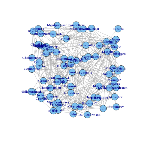
The co-appearance network of characters from Victor Hugo's novel Les Miserables, from D. E. Knuth, The Stanford GraphBase: A Platform for Combinatorial Computing, Addison-Wesley, Reading, MA (1993), is a classic example network.  It is certainly commonly used: for example, here, here, here, here, here, here, here, here, here, and here!  Those links lead to a variety of different visualizations, including adjacency matrices, arc diagrams, and many node-link diagrams with different types of layouts.  So as a first example, I have created a BioFabric version of that network, shown in this thumbnail:

Click on image to enlarge

Click on the thumbnail above to view the network, or go take a look at the much larger version available at the newly-created BioFabric Gallery.  Even better, you can get the BioFabric .bif file from the Gallery as well and load it into BioFabric to explore the network interactively.  For while this network may be small enough to make it practical to use just a static image, the interactive viewer is really essential as networks grow in size.  And I can't stress enough how important interactivity is with BioFabric!  Being able to pan over the entire network, and zoom in to view interesting features, is a key aspect of the working with a BioFabric network.

The GML file for this network that is available from the Gephi Datasets Wiki includes cluster assignments for the nodes, and these have been used to create the clustered layout shown above.  Note the following things about this layout:

• The clustered layout technique used above is not yet built into BioFabric Version 1.0.0, so the ordering of node rows and edge columns was calculated externally, then imported.  Getting this technique built into the program is high on the list of planned enhancements. 
• The clusters were ordered from top to bottom according to the number of nodes in each cluster.
• Each cluster was first laid out separately using just the intra-cluster edges and the default breadth-first search technique. The inter-cluster edges were then added, and assigned to columns so that connections between clusters are visually distinct from the edges within each cluster.   There was then a final step of manual tweaking to fine tune the layout.
• There are several cliques in this network, e.g. the Fantine and most of the Marius clusters, and they stand out in this layout as a series of adjacent edge wedges of steadily decreasing size.

So there is now yet another way to look at this venerable network example!  If you have any questions, please add them in the comments.